Trimming my Grass Shader
• By: Aleksandar Gjoreski
At the end of last year, on New Year’s Eve, I published Growing my Grass Shader, and soon after, things here went a bit quiet.
Back in January a friend and I had started building something of our own, chasing the idea of turning a shared dream into something real, closer to maths and civil engineering than to 3D worlds :)
That project is still going strong, and it took most of my time for a while.
I enjoy working on it and I keep learning a ton, but I really needed a change of context.
Coming back to Revo meant coming back to 3D graphics, where I can experiment freely, express myself creatively and generally feel much more at home.
Fresh eyes also made me notice quite a few things I had ignored or simply missed before.
Some of that work had very little to do with grass directly. I spent some time separating the render and physics schedules as well as replacing the diagnostics tool I had with something built around Revo itself, even though the monitoring is not perfect yet. For example, I am still not measuring real CPU and GPU frame time the way I would like, but I know where the numbers come from and can extend the system whenever and however I need.
It gave me more control over the whole project and helped me see what the grass was doing much more clearly.
That is why this grass article starts there, even if it wasn’t the first thing I touched after coming back to the project.
Before getting into any of that, this is where Revo is at the time of writing:
The chapters below continue from where the previous article stopped because this is pretty much the next part of the same story.
The flip in the title is a wink at where all of this is actually going ;)
9. Tick-tick, tock-tock, pick a clock
Timing had already caused a few problems.
At some point Revo had behaved differently between my 120 Hz and 165 Hz monitors. I had already fixed that particular speed difference before this rework, but it was still a good reminder of how fragile timing can become when too many things depend on the same update.
Halving the frame rate, which was the only knob I had at first, introduced some visible stutter, even when the physics itself remained stable.
Rendering was the part I really wanted to control properly. Separating it from the rest of the loop also made me look at physics more carefully.
It became much easier for me to reason about the loop once I stopped treating rendering and physics as if they followed the same clock.
I was already using a fixed-step accumulator with interpolation. This rework let those physics steps run independently from the rendering schedule and gave time, physics and rendering a much clearer role in the loop.
The orchestrator
The main loop is small and simple on purpose. It helps me see what happens step by step at a glance.
Every display update gives physics a chance to process the time it is owed, while rendering continues only when FrameScheduler
allows it.
This is how those pieces are orchestrated:
// both are { delta, player }; physicsState.delta is always the fixed 1/60 step
onAnimationFrame = (timestamp: DOMHighResTimeStamp) => {
  timeManager.update(timestamp);
  if (timeManager.isPaused) return;

  physicsScheduler.update(timeManager.delta);
  for (let i = 0; i < physicsScheduler.pendingSteps; i++) {
    eventsManager.emit("engine-before-physics", physicsState);
    physicsManager.step();
    eventsManager.emit("engine-after-physics", physicsState);
    physicsManager.flush();
  }

  frameScheduler.update();
  if (!frameScheduler.shouldRender) return;

  renderState.delta = timeManager.consumeRenderDelta();
  eventsManager.emit("engine-render-update", renderState);
  rendererManager.render();
  monitoringManager?.sample(timestamp);
};- Time →
TimeManagermeasures and accumulates the elapsed time. - Physics →
PhysicsSchedulerdecides how many fixed steps are owed, thenPhysicsManagerexecutes them. - Rendering →
FrameSchedulerdecides whether to draw, thenRendererManagerdoes the actual rendering.
EventsManager connects everything else to the relevant physics and render phases, so the loop does not need to know that grass,
wind, the player or any other particular system exists.
Skipping a render also does not throw its time away. TimeManager keeps accumulating it, then consumeRenderDelta() gives the
complete amount to the next render update. Anything animated from render delta therefore continues at the correct speed even when
the scheduler draws less often.
You might think: “So many managers…managing…stuff”. Fair :)
The
forloop inside a frame update may look a little scary at first, but it only processes the fixed physics steps currently owed, and it can run at most four times (deliberate cap on my end). Based on what I have experienced, during normal 120 Hz rendering, most display updates owe either zero or one.
Physically fit
The fixed-step accumulator itself was already in Revo before this rework.
Physics generally behaves better when every update represents the same amount of simulated time. Real frames can arrive early or late, but the solver continues moving through equal steps instead of receiving a different-sized jump every time.
I kept Rapier’s default 1/60 step.
It is a familiar compromise for this kind of simulation: frequent enough for Revo’s movement and collisions, without running physics 120 times per second just because my laptop display can render that often.
The scheduler stores whatever time has not been simulated yet in an accumulator:
const FIXED_DELTA = 1 / 60;
const MAX_STEPS_PER_FRAME = 4;

export class PhysicsScheduler {
  private accumulator = 0;
  pendingSteps = 0;
  fixedDelta = FIXED_DELTA;

  get alpha() {
    return this.accumulator / this.fixedDelta;
  }

  update(delta: number) {
    this.accumulator += delta;

    const owedSteps = Math.floor(this.accumulator / this.fixedDelta);
    this.pendingSteps = Math.min(owedSteps, MAX_STEPS_PER_FRAME);

    this.accumulator -= this.pendingSteps * this.fixedDelta;
    if (this.accumulator > this.fixedDelta) this.accumulator = this.fixedDelta;
  }
}
If less than one step is available, physics waits. If enough time has accumulated for two, both are processed before rendering. At normal speed this averages out to 60 physics updates per second regardless of whether the scene renders at 120, 60 or 40 FPS.
Pause and slow motion intentionally change the rate against wall-clock time, but each simulation step remains 1/60 of a second.
TimeManager clamps an incoming frame delta to 1/15 of a second, roughly 66.7ms, and PhysicsScheduler allows at most four
1/60 steps in one frame.
The numbers match on purpose: both limit catch-up to roughly 66.7ms.
After those steps are removed, the final check prevents more than one step of debt from remaining in the accumulator, so a long stall cannot keep building a larger backlog across the frames that follow.
The remaining fraction is exposed as alpha. The player uses it to interpolate its visual position between the previous and
current physics snapshots:
this.visualRoot.position.lerpVectors(
  this.prevPosition,
  this.targetPosition,
  physicsScheduler.alpha,
);
Here
visualRootis just anObject3Dwrapping the player’s mesh, which lets me easily control squishing and other effects.
The rigid body stays on the fixed simulation while only visualRoot is interpolated. That keeps movement smooth when the physics
and render clocks do not land together, especially at the lower frame rates where I had noticed the stutter much more easily.
Summertime Rendering
The render side is tied to a different rhythm: the display refresh.
On my 120 Hz laptop, rendering every refresh gives me 120 FPS. Rendering every second refresh gives me 60, every third gives me 40 and every fourth gives me 30.
All of those divide evenly into 120, so the time between rendered frames stays consistent.
Asking for 80 FPS would not divide cleanly. Some frames would remain on the screen for one refresh and others for two, which can feel less smooth even if the average still says 80.
FrameScheduler therefore works with a divisor:
update() {
  this.displayFrame++;
  this.shouldRender = this.displayFrame % this.divisor === 0;
}
The system measures the display first because the browser does not expose a reliable refresh-rate property. It collects 61
consecutive animation-frame timestamps, ignores intervals longer than 50ms, takes the median of the remaining deltas and snaps
the result to a list of common display rates.
Once it knows the refresh rate, ceil(refreshHz / targetFps) produces the divisor.
The target is therefore treated as a maximum. A target of 120 on a 120 Hz display stays at 120. On a 165 Hz display the same target
produces a divisor of 2, so the effective rate becomes 82.5 FPS instead of trying to fit an uneven 120 into 165 refreshes.
60 FPS was always a perfectly reasonable fallback, and it is still the familiar smooth baseline for most things. But I knew Revo could comfortably run at 120 if I managed to reduce the grass overhead, so settling for 60 was a little bit frustrating.
Press F
I had been using stats-gl since the beginning. It was the first thing I used to see what Revo was doing.
Alongside some of its built-in panels, I slowly added custom ones for things like draw calls and the number of triangles in the scene, until it grew into a fairly decent monitoring setup.
The issues started when I wired up postprocessing.
Without it, its GPU numbers looked reasonable for what was still a mostly empty world. I had no way to verify whether they were correct, but at least they looked believable.
With postprocessing enabled, GPU time jumped above 25ms and kept producing large spikes while the scene itself remained smooth.
Maybe there was a valid explanation somewhere in the way the work was measured, but the result was misleading enough that I
eventually disabled that panel.
For a while, FPS was the only built-in panel I still used alongside my custom ones.
Once I had built the scheduler and already owned the target and effective rates, keeping an entire third-party library for that one number felt unreasonable, so I thanked it for its service and uninstalled it.
The replacement is a small MonitoringManager (exactly, yet another manager) that gathers one snapshot per second.
It already shows quite a few things: the current, target and effective FPS, the render interval against its budget, late frames, display refresh and divisor, interpolation alpha, and more.
On top of that, I can also easily wire up any extra information registered by another system such as grass.
It’s not perfect, of course.
What the panel calls Average shows the average interval between rendered frames over the last second, while Budget shows what
that interval should be at the effective FPS, for example: 8.33ms at 120 FPS or 16.67ms at 60. Any interval exceeding it by
more than 1ms counts as late.
These values describe render cadence, not CPU or GPU execution time.
Frame time is more useful than FPS for finding individual problems, but I am not quite measuring it properly yet and I do not want to pretend otherwise. What I have now is closer to what I need, built around Revo and completely under my control. I know where the numbers come from, and I can change or extend the system as I understand more.
The culling work later in the article added a provider for the rendered and total blade counts. MonitoringManager receives them
asynchronously and uses them to correct the global triangle count. I had the grass use case in mind from the beginning, but I kept
providers generic enough for other systems to contribute too.
Having that control makes me much more confident about working on the actual world now.
There is still plenty for me to learn and improve, but Revo keeps becoming more robust as I do :)
10. Rolling the dice properly, finally
The first grass problem I touched after returning to Revo was a strange little growth effect.
While moving around, every now and then I would catch a blade growing from almost nothing back to its full height over a few frames. It was quick, it did not happen everywhere and following it on purpose was considerably harder than spotting it from the corner of my eye.
This capture is slowed down because the real effect was much easier to miss:
Blades casually growing into existence (3x slower capture)
My first suspect was the trail system. Grass touched by the player gets crushed by reducing its scale, then slowly recovers to its original height. If that scale somehow ended up on a blade that had just appeared, the result would look exactly like what I was seeing.
Checking the trail exposed the first issue in the wrapping logic.
The grass field follows the player, reusing the same buffer slots as blades wrap from one side to the other. A slot carrying a crushed blade could therefore move to a completely different place while its scale was still recovering.
I ended up separating movement from wrapping, which also made that exact moment much easier to detect. unwrappedOffset is where
the slot would land after applying the player’s movement, while the mod() on each axis only folds it back inside the grass field:
const previousOffset = vec2(data1.x, data1.y);
const unwrappedOffset = previousOffset.sub(uniforms.uPlayerDeltaXZ);
const wrappedOffsetX = mod(
  unwrappedOffset.x.add(config.TILE_HALF_SIZE),
  config.TILE_SIZE,
).sub(config.TILE_HALF_SIZE);
const wrappedOffsetZ = mod(
  unwrappedOffset.y.add(config.TILE_HALF_SIZE),
  config.TILE_SIZE,
).sub(config.TILE_HALF_SIZE);
const wrappedOffset = vec3(wrappedOffsetX, 0, wrappedOffsetZ);

const wrapDelta = wrappedOffset.xz.sub(unwrappedOffset);
const isWrapped = step(
  config.TILE_HALF_SIZE,
  max(abs(wrapDelta.x), abs(wrapDelta.y)),
);
Most frames wrappedOffset.xz and unwrappedOffset are identical, so wrapDelta is 0. Once a blade crosses an edge, the modulo
shifts it by one full tile. step() turns that jump into the 0/1 flag I need, and the comparison still works if a larger
movement crosses more than one tile at once.
Whenever isWrapped is 1, that buffer slot now represents a different patch of ground. Resetting its scale to the base value of
the new location got rid of the most obvious version of the growth.
I could still catch the effect here and there though. Since it only became visible after a blade disappeared and came back, I followed the other part of the chain that can do exactly that while the blade is still inside the camera: stochastic thinning.
That exposed another wrapping mistake and gave me a good excuse to improve the keep decision while I was already there.
A stable seed
Stochastic thinning gives every blade a keep probability called p. Nearby blades get a value close to 1, distant ones move
towards pMin, and each blade compares that probability with its own random roll:
const p = mix(1, pMin, t);
const rnd = hash(float(instanceIndex).mul(0.73));

const keep = step(rnd, p);
step(rnd, p) returns 1 when p reaches or passes the roll, otherwise it returns 0 and the blade is dropped.
I used instanceIndex as the seed because the same index always produced the same roll. I even described the result as stable
under wrapping in the previous article.
The number was stable, sure. instanceIndex itself belongs to a reusable slot in the grass buffer though, not a fixed place in the
world. Slot 42 may represent one patch of ground now and another one after wrapping, while its roll follows it to the new location.
That new patch could therefore receive a completely different keep decision even if its distance from the player had barely changed.
Another little source of popping to fix while I was already there.
The roll needed to belong to the patch of ground instead. Dividing the world position by the spacing between blades gives me a stable grass cell, whichever buffer slot happens to represent it:
const cell = floor(worldPos.xz.div(spacing));
const rnd = hash(cell.x.mul(12.9898).add(cell.y.mul(78.233)));
Those constants only mix the two cell coordinates before the hash. The important part is cell: the slot may change after
wrapping, but the patch now receives the same roll.
A flickering situation
While I was already inside the keep function, distance alone did not feel like enough. Two blades can be equally far from the player and contribute very differently to the final image depending on their height and the camera.
I added a rough estimate of the blade height on screen. fY comes from the camera projection and clipPosition.w gives me its
depth. Their ratio is enough to estimate the projected height without doing anything particularly expensive.
That estimate becomes pScreen: near 0 while the blade is tiny on screen and 1 once it is large enough to receive the full
distance probability. Multiplying the two gives the final p.
Adding projected size also made the decision more sensitive. The player moves, the camera moves, the depth changes, and p may end
up hovering around the blade’s random roll. One small movement puts it above the roll, another puts it below, and the blade keeps
changing its mind.
Have you ever tried to balance a light switch exactly in the middle? Well, I surely did, and of course, exactly as one might expect: I couldn’t.
Turns out, snap-action light switches are a very practical example of hysteresis. Instead of using one threshold in both directions, they have one point where they switch one way and another where they switch back.
Imagine a threshold of 15 with a hysteresis of 5. Moving upwards, the state changes when the value reaches 20. Moving back
down, it only changes after falling below 10. The full gap is therefore 10, exactly twice the hysteresis value.
A value bouncing between 15 and 16 can no longer make the state fight back and forth. Once it has crossed 20, it remains
there until it drops below 10.
In my case, with rnd = 0.60 and hysteresis = 0.11, a hidden blade needs p to reach 0.71 before it appears. Once visible, it
remains there until p falls below 0.49.
There is no longer one switching point I could somehow balance on. After falling below 10, moving back to 11 is not enough to
switch again, and the same happens at 20 when moving back to 19. That point does not exist, which also explains why
balancing a light switch was a lost battle from the beginning.
The spring-loaded mechanism inside the switch makes the physical version even more obvious by snapping the lever towards either side, but the hysteresis already made the switching boundary itself impossible to balance.
Hysteresis needs to know whether the blade was visible in the previous frame. That state belongs to the old grass cell after
wrapping though, so I clear it whenever isWrapped is 1:
const previousKeep = wasVisible.mul(float(1).sub(isWrapped));The new location therefore starts with previousKeep = 0 and has to make its own enter decision.
Put together, with t still being the 0..1 distance remap from the previous article, the keep function now looks like this:
const pDistance = mix(1, pMin, t);

const eyeDepthAbs = clipPosition.w.abs().max(EPSILON);
const projectedBladeHeight = fY.mul(bladeHeight).div(eyeDepthAbs);
const pScreen = smoothstep(projectedMin, projectedFull, projectedBladeHeight);

const p = pDistance.mul(pScreen);

const cell = floor(worldPos.xz.div(spacing));
const rnd = hash(cell.x.mul(12.9898).add(cell.y.mul(78.233)));

const enterThreshold = rnd.add(hysteresis).clamp();
// keep it above 0, otherwise step(0, 0) returns 1 and keeps the blade
const stayThreshold = rnd.sub(hysteresis).clamp(EPSILON, 1);

const enterKeep = step(enterThreshold, p);
const stayKeep = step(stayThreshold, p);

return mix(enterKeep, stayKeep, previousKeep);
When previousKeep is 0, mix() selects enterKeep and the blade has to cross the higher threshold. When it is 1, it selects
stayKeep and the blade remains until it crosses the lower one.
p never leaves the 0..1 range, so neither threshold should. Clamping the enter threshold means every blade can still appear
when p reaches 1. Starting the stay threshold at EPSILON gives us the opposite boundary: when p reaches 0, every blade
leaves.
The roll now stays with the patch of ground, the probability also accounts for how large the blade is on screen, and hysteresis stops it from flickering around the threshold.
Full circle
The thinning looked considerably calmer after all of that, especially around wrapping and the enter/exit thresholds. I could still catch the original growth effect though.
The full sequence was:
- The trail crushes a blade by reducing its stored scale.
- Stochastic thinning hides it before the recovery finishes.
- The blade no longer enters the remaining update work, so recovery pauses at that partial scale.
- Stochastic thinning admits it again and the same partial scale comes back with it.
- The material draws the blade while the following frames finish the recovery on screen.
The compute shader has two visibility gates. The first one combines the frustum and stochastic decisions:
const wasVisible = getVisibility(data1);

const passesStochasticThinning = computeStochasticKeep(/* ... */);

const isInFrustum = computeFrustumVisibility(/* ... */);

const isPotentiallyVisible = isInFrustum.mul(passesStochasticThinning);
data1.assign(setVisibility(data1, isPotentiallyVisible));
Every blade has to reach those checks. Only the ones that survive both enter the first If, where I sample the grass map and work
out their final scale:
const originalScale = getOriginalScale(data1);

If(isPotentiallyVisible, () => {
  // terrainMaps -> R = baked shadows, G = grass, B = water
  const maps = texture(terrainMaps, computeMapUvByPosition(worldPos.xz));

  const grassScale = maps.g;
  const baseScale = originalScale.mul(grassScale);
  const isVisible = step(config.MIN_VISIBLE_SCALE, baseScale);

  data1.assign(setVisibility(data1, isVisible));

  If(isVisible, () => {
    // ...terrain height, trail, wind, shadow and compaction
  });
});
baseScale combines the blade’s original random size with the value painted into the grass map. The small
MIN_VISIBLE_SCALE cutoff removes almost-flat blades around its edges.
The second If is worth keeping even if most candidates pass it. Anything rejected there skips the terrain height, trail, wind,
shadow and compaction work. We will get to that last part in chapter 12. Sampling the grass map before the first gate would make
all 1M blades pay for it instead.
That is exactly where the stored scale was getting stuck. Once a blade fails the first gate, its trail recovery no longer reaches the buffer. The scale stays exactly where it was until the blade becomes visible again.
I had already saved the previous visibility before either gate wrote a new value. Together with the current stored scale, the missing reset ended up being quite small:
const currentScale = getScale(data1);

const recoveredScale = mix(currentScale, baseScale, uniforms.uTrailGrowthRate);

const didAppear = isVisible.mul(float(1).sub(wasVisible));
const shouldReset = max(isWrapped, didAppear);
const scaleBeforeTrail = mix(recoveredScale, baseScale, shouldReset);
didAppear becomes 1 when the blade is visible now after being hidden in the previous frame. shouldReset also includes
isWrapped, since a wrapped slot belongs to a new patch of ground even if it happened to remain visible through the move.
For blades that stayed visible, scaleBeforeTrail keeps the usual gradual recovery. Newly visible or wrapped blades use
baseScale immediately instead of carrying a stale partial height into the new frame.
The same flag also resets the previous wind bend before the remaining work continues:
If(isVisible, () => {
  const nextScale = mix(
    scaleBeforeTrail,
    crushedScale,
    uniforms.uKDown.mul(contact),
  );
  data1.assign(setScale(data1, nextScale));

  const newWind = computeWind(
    previousWind,
    worldPos,
    positionNoise,
    shouldReset,
  );

  // ...shadow and compaction
});
That was the last case I was missing. Once wrapped slots and newly visible blades both started from the right state, I could no longer reproduce the growth effect.
Somewhere to play
Revo became a football very early in the project. It was not its original design, technically, but it has been one almost since the beginning.
Football has always been much more than just a sport to me personally.
Once Revo became something I could kick and roll around, I naturally wanted to give it somewhere proper to do that.
The recent World Cup only added to that excitement. I enjoyed it very, very much, watching matches even at 2 AM despite having to work the next day. It was wonderful.
I wanted a small pitch with short, nice-looking grass, painted lines, proper goals and… more ;)
The shorter grass was the first part, and achieving it turned out to be quite simple once I removed my blinders.
You may have noticed that the code above now turns that sample into grassScale instead of a visibility test. Underneath, it is
still the exact same sample from the same green channel of terrainMaps. The value had always been continuous between 0 and 1;
I was simply reducing it to a yes or no instead of using it to control the height.
The texture was not missing anything. I was consuming it the wrong way.
I still need to find a nice and neat way to paint the lines, apart from the obvious answer, although perhaps I can use one of the channels already sitting there. We will see.
I love this game!
Patrice Evra
11. A wind from the East
About two years ago I played Ghost of Tsushima for the first time.
I had already seen screenshots and clips from other people’s playthroughs, and those were what first inspired the grass field. Playing it myself was a completely different story though.
I could stop almost anywhere just to admire the scenery, which happened quite often because the game made almost everywhere worth looking at.
Among everything that made me fall in love with it, the guiding wind is still one of my favourite features.
It simply looked beautiful! It was genuinely useful and it let the HUD stay remarkably clean.
Swipe upward and the world itself points towards your destination. No line painted on the ground and no marker asking to be followed every second.
At the time of writing, I am playing Ghost of Yotei, which uses the same mechanism, but Tsushima is where the idea came from for me.
Revo already had directional wind around the time I shared the previous article. The idea of making it visible with particles and lines had been there since I first added it. I just kept postponing that part until now.
That shared directional wind is also what connects this little detour back to the grass. The particles and streaks are new, but they all move as part of the same gust.
One wind to rule them all
Before the WindManager, trees, flowers and grass each had their own version of wind. They could all move, but there was no shared
directional event feeding them the same information.
The manager filled that gap. It runs on the CPU, owns the direction and intensity, then exposes them as TSL uniforms that shaders across Revo can consume:
export class WindManager {
  readonly uDirection = uniform(new Vector2(0, -1));
  readonly uIntensityDirectional = uniform(0);

  // ...
}
Selecting a discovered landmark gives WindManager a target, and a trackpad swipe up starts four simple phases:
- Calculate direction → Point from the player’s current position towards the selected landmark.
- Ramp intensity → Smoothly increase the directional wind until it reaches full strength.
- Hold → Keep it there for 3 seconds.
- Decay → Gradually bring the directional intensity back to zero.
The direction is calculated once when the gust begins. Moving during those few seconds does not rotate it halfway through. Once it ends, another swipe calculates a fresh direction, while reaching the landmark clears the target automatically.
Grass, flowers, particles and streaks all receive that same direction and intensity. Each system still decides how much it bends, how fast it moves and what full strength means for it.
One might rightfully ask: “Why didn’t you also mention trees?”
Fair question. Sharp eyes. Their shadows are currently baked, and making the trees sway much more than a subtle oscillation would most likely break the illusion. Maybe in the not so distant future…who knows.
Volumetric air
The names moved around a little while I worked on this. They started as lines, the longer version became ribbons, and the shorter trails I eventually kept are now streaks. Apparently even naming them needed a few passes :)
The current visual layer is made of sprite particles and 12 streaks.
I see the small particles as pollen or dust giving some volume to the air. The streaks are the readable part of the gust: long, soft strokes making the direction obvious without adding an arrow to the screen.
Guiding wind in Ghost of Tsushima - by Hijacked Games
The particles are much simpler. I spread 4,096 of them around Revo in a 64 × 64 grid. Every particle receives a stable
little offset, while its position and age stay inside a vec4 SSBO.
The field follows the player and wraps at its edges in a similar way grass does. When a particle reaches its lifetime, it respawns from the side the wind is coming from, while the wind direction and a little noise keep it moving in a less regular way.
A stable hash makes them scale in and out at slightly different moments during a gust, so the air fills up gradually instead of everything appearing at once.
One curve, twenty-five points
The streaks took a few attempts, visually and technically.
Ghost of Tsushima was the inspiration for both the idea and the look, but I still wanted to tailor it to Revo. The final version is shorter and a little more playful than the big guiding wind strokes in Tsushima. I think it fits better in this small world.
Each of the 12 streaks starts as a very small piece of state stored in an SSBO: where its curve begins, how far it has travelled
along that curve, and a shared height for the whole streak, smoothed over time so it glides up and down instead of snapping to the
terrain.
The plane is divided into 24 segments along its length. This gives it one starting edge, 23 internal ones, and one ending edge,
for a total of 25.
Each edge connects two vertices, one on either side of the strip. The compute pass calculates only its midpoint, and the material then uses that midpoint to position the two vertices in opposite directions and give the streak its width.
This way, I only need to store 25 midpoint positions instead of 50 individual world-space vertex positions.
When the player swipes to call the wind, WindManager starts a gust and the streaks are placed around the field. During the
gust, the compute pass moves them with the shared direction and intensity, each with a small stable speed variation so they do not
all march across the screen together.
The path itself is simple. It moves forward in the wind direction while a sine wave bends it sideways a little. That same pass then
calculates 25 points along the curve, each one a little further behind its front.
The terrain underneath the front of the streak, together with its individual height offset, provides a target for its shared height. Instead of adopting that value immediately, the height moves towards it gradually, letting the whole stroke glide up and down.
Every midpoint starts from that smoothed height but still checks the terrain directly underneath it. If the terrain plus a small clearance is higher, that point is lifted just enough to stay above it. This keeps the streaks clear of hills without making them stick rigidly to every bump in the ground.
const sharedHeight = mix(previousHeight, targetHeight, smoothing);
const pointHeight = max(sharedHeight, terrainHeight.add(clearance));
Once a streak travels far enough, the compute pass places it back behind the player and rebuilds its points from there.
The material uses the neighbouring midpoints to find which way the curve is heading. It then uses the camera direction to find the corresponding sideways axis and places the two vertices along it. This keeps the strip facing the camera.
When the camera looks almost directly along the streak, the view and curve directions become nearly parallel, so they can no longer provide a reliable sideways axis. The fix is quite simple: the material uses the world’s fixed upward direction instead to work out where the two sides should go.
Tighter bends create a separate problem because the two sides can collapse towards each other. Slightly increasing the width around those bends keeps the strip from pinching.
Also worth noting: I tried SpriteNodeMaterial briefly.
On paper it looked like it could take care of the camera-facing part for me, but I struggled to make it work properly with all the
rest. It also took my stable 120 FPS down to around 105 in that experiment. Not great.
That may well have been my implementation rather than the material itself, but I was not going to keep it around just to prove a point.
The custom MeshBasicNodeMaterial is a little more hands-on, but fairly simple now. The streaks look right and the frame rate stays
nice and stable where I want it.
Easy decision.
And this whole wind system I built? Purely out of love for someone else’s game :)
12. GPU culling: atomic compaction
Alright, finally, the juicy part :)
Before real GPU culling, I was already reducing the amount of grass that could make it to the fragment shader through a chain of three checks:
- Frustum culling → reject blades outside the camera
- Stochastic thinning → gradually draw fewer blades further away
- Grass map → reject blades whose resulting scale falls below a small threshold
All three eventually produced one flag: isVisible.
The compute shader used it to skip most of the heavier work for rejected blades. The material also moved the blades dropped by stochastic thinning and the grass map outside the frustum, since those could still be on screen and create overdraw otherwise.
This helped quite a lot. Every draw still started with all 1M blades though, so the GPU had to begin the vertex work for each one before the material could move the rejected ones away.
My target for Revo has always been at least 120 FPS, mostly because that is the refresh rate of the laptop I use to build it and I really like how smooth it feels there. Most of the time it stayed around that target quite comfortably.
While wandering around the map I did notice a few small hiccups every now and then though, and unfortunately I never managed to find a pattern behind them.
The bottom-left corner of the map, close to the lake, was much easier to reproduce. It usually stayed around 105 to 110 FPS but could drop as low as 100. The “good” part was that the final build, without monitoring or debugging hooked up, ran smoothly enough for those drops to be basically unnoticeable on my machine.
I still knew they were there in development though. Revo is also far from finished, so carrying that overhead into everything I still want to add did not sound great.
I did try to send fewer vertices first by reducing the number of segments in each blade. It helped a bit, but not enough to justify how much the look changed once I pushed it further. I had pictured the grass as that soft, fluffy carpet since the beginning, and reducing the blades to what were basically triangles did not match that at all.
So I went after the blade count instead.
The CPU could not cull individual blades because it knew basically nothing about them. Their positions, wrapping and visibility all lived on the GPU. I could move the whole thing back to JavaScript and finally give the CPU enough information, though processing 1M blades there just to make the draw cheaper felt like a wonderful way to achieve the opposite.
So… GPU culling it was. I had tried that once already, and my choice of route looked more or less like this:
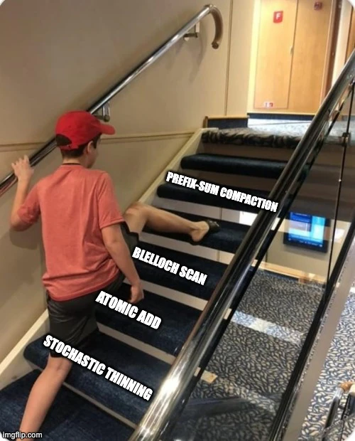
I dismissed the atomic solution almost immediately. Thousands of GPU threads competing for the same value sounded like an obvious bottleneck, so naturally I skipped it and jumped straight to prefix-sum compaction instead.
Basically me walking directly into the final boss because it looked fun (and because I can be stubborn sometimes), just to get humbled fairly quickly.
I already had the visibility decision in isVisible, so the atomic route was conceptually much simpler than prefix-sum
compaction: if a blade was visible, it claimed a place in a new list and wrote its index there.
I still had the same prejudice about the simpler solution, but I decided to give it a shot anyway before deciding it was a bottleneck, and it proved me wrong.
It actually worked great.
A ticket machine for grass
A ticket machine is probably the simplest analogy here. The blades queue around one shared counter, where each one receives a unique number that becomes its position in the list of visible blades.
It does not matter who gets served first. I only need the numbers to start at 0, contain no gaps and never be handed to two
blades at the same time.
The operation behind all of this is atomicAdd:
const visibleBladeIndices = instancedArray(config.COUNT, "uint");

// ...all the previous grass work

If(isVisible, () => {
  // ...trail, wind and shadow updates

  const drawIndex = atomicAdd(atomicCounter, 1);

  // save the original blade index at its new compacted position
  visibleBladeIndices.element(drawIndex).assign(instanceIndex);
});

// ...
When a blade calls atomicAdd, it receives the current value of the counter and increments it by 1 as part of the same operation.
If the counter contains 17, that blade receives slot 17 and leaves 18 for the next one. The whole thing is atomic, so another
thread cannot receive 17 too.
instanceIndex is the blade’s original index in the complete field. drawIndex is its new position among the blades that survived.
If A, C, D, G and H are visible, the threads could reach the counter in any order and produce something like this:
original:   A  B  C  D  E  F  G  H
visible:    1  0  1  1  0  0  1  1
compacted:  A  D  H  C  G  *  *  *
count:      5

* means whatever was there before, it doesn't matter
There is no point in preserving their original order here. The valid part of the list has no gaps, no two blades write into the same place and the counter already contains the number of blades I need to draw.
Every frame begins by clearing one value: that counter.
computeResetInstanceCount = Fn(() => {
  atomicStore(atomicCounter, 0);
})().compute(1, [1]); // one counter only needs one thread
atomicStore replaces the value instead of incrementing it. I do this in a separate one-thread compute pass because putting the
reset inside the grass update could let one workgroup clear the counter while another was already using it. There is no global
barrier inside one dispatch that could make every workgroup wait for the reset first.
The foundational rework introduced earlier lets me keep that order explicit:
const computeTask = rendererManager.createComputeTask({
  label: "Grass",
  init: ssbo.computeInit,
  update: [
    ssbo.computeResetInstanceCount, // always reset first
    ssbo.computeUpdate, // then rebuild the visible list
  ],
});
I do not clear the compacted list itself. Every visible blade overwrites one slot starting from 0, and the final count limits the
draw to exactly those slots. If one frame writes five indices and the next one writes only three, anything after the third slot is
simply unreachable.
Connecting the dots
I now had the exact count and a compacted list of the blades that survived. I could read that count back into JavaScript every frame and update the mesh from there, but that would put the CPU right back in the middle.
CPU and GPU normally keep working without waiting for one another. A readback introduces a synchronization point because the CPU cannot use the value until the GPU has finished writing it. Unified memory may remove a physical transfer, but it does not remove that wait. I would then send the exact same number straight back to the GPU with the next draw call.
Quite the detour. An indirect draw removes it.
With a normal draw, the CPU gives the GPU the arguments, including how many instances to draw. An indirect draw reads those arguments from a GPU buffer instead.
Since the compute shader already produced the visible count there, the draw can use it directly without reading anything back into JavaScript.
Three.js provides an IndirectStorageBufferAttribute construct that makes it easy to wire it up with a geometry. Here is how I
set it up:
const indirectDrawAttribute = new IndirectStorageBufferAttribute(
  new Uint32Array([
    config.BLADE_INDEX_COUNT, // indexCount
    0, // instance count, updated every frame by the atomic counter
    0, // firstIndex
    0, // baseVertex
    0, // firstInstance
  ]),
  1, // size of each argument, all of them are uint so 1
);

const atomicIndirectDrawArguments = storage(
  indirectDrawAttribute,
  "uint",
  indirectDrawAttribute.count,
).toAtomic();

// instance count is the second indirect draw argument
const atomicCounter = atomicIndirectDrawArguments.element(1);indexCount→ how many indices make one blade (mine uses21at the time of writing)instanceCount→ how many blades to draw (this is the counter)firstIndex→ where to begin in the geometry’s index bufferbaseVertex→ an offset added to the vertex indices (I do not need one)firstInstance→ where to begin in the available instances
The counter is not copied into this buffer afterwards. atomicCounter is an atomic TSL reference to its second value from the
beginning, so both atomicAdd and atomicStore update the exact memory the draw later reads as instanceCount. The other four
values never change.
storage(...).toAtomic() does not create another GPU buffer. It exposes the existing indirect attribute to the compute shader
with atomic access, then .element(1) selects the counter.
One small detail here is that
toAtomic()marks the whole five-value storage view as atomic, even though I only use atomic operations oninstanceCount. TSL models this version as one homogeneous array, so all its elements need the same type. I could have described the indirect arguments as a customstructand marked only that field atomic, but that would also mean maintaining another exact description of WebGPU’s layout for no practical benefit here. The other four values do not suddenly start doing atomic work simply because they are declared that way.
Strictly speaking, baseVertex is signed while the other four values are unsigned. Mine is 0 though, so using a Uint32Array
does not change anything here.
The first version of GPU culling was already working great with the InstancedMesh I had been using since the beginning.
When I checked the setup again though, passing COUNT to the mesh first and then letting the indirect buffer provide the actual
count for the draw felt a bit strange.
I dug into whether a regular Mesh with InstancedBufferGeometry could do the same job and what the difference would be. The
regular Mesh version worked exactly the same. That small detour also led me into the Three.js source, where InstancedMesh
creates an instanceMatrix with count × 16 floats. Revo never used those matrices because every blade position came
from the SSBO. Each matrix still took 64 bytes though (16 floats at 4 bytes each), which added up to roughly 67 MB of unused
CPU-side memory across the whole field.
Not exactly peanuts, so definitely a very welcome saving.
So I switched the blade geometry to InstancedBufferGeometry and used a regular Mesh instead:
export class GrassBladeGeometry extends InstancedBufferGeometry {
  // ...blade geometry
}

const geometry = new GrassBladeGeometry({
  nSegments: config.SEGMENTS,
  bladeHeight: config.BLADE_HEIGHT,
  bladeWidth: config.BLADE_WIDTH,
});

geometry.instanceCount = config.COUNT; // logical maximum; the indirect draw supplies the current count
geometry.setIndirect(ssbo.indirectDrawAttribute);

const mesh = new Mesh(geometry, new GrassMaterial(ssbo));
geometry.instanceCount = config.COUNT keeps the complete field as the logical maximum. For a normal instanced draw, that is the
count Three.js would use. Once the WebGPU backend sees the indirect attribute, it issues drawIndexedIndirect instead and reads
the current count from the GPU buffer.
The indirect attribute belongs to the geometry because those arguments describe how the geometry should be drawn: how many
indices to use, where to begin and which offsets to apply. InstancedBufferGeometry already makes the draw instanced, so a regular
Mesh is enough and I do not need 1M standard matrices just to get instanceIndex.
The draw was compact now, which meant instanceIndex no longer referred directly to the original blade. It only told me which
slot of the compacted list I was drawing. Draw instance 12, for example, was not necessarily the original blade 12 anymore.
// compacted draw index -> original blade index -> persistent blade data
const bladeIndex = visibleBladeIndices.element(instanceIndex);
const data1 = computeBuffer1.element(bladeIndex);
const data2 = computeBuffer2.element(bladeIndex);
I read the real blade index from that slot first, then use it to access the same SSBO data as before.
Pretty simple in the end.
Was it worth it?
TL;DR: I think so!
The compute pass still starts one thread for every blade. As explained in the previous article, rejected blades leave before the later trail, wind and shadow work. Now they also stay out of the vertex stage completely. There is still some compute work attached to them though.
The monitoring panel reads the final count asynchronously once per second, only so I can see what the GPU decided. Rendering never waits for that diagnostic readback.
The visible count reaches around 250k blades at most in the densest views, meaning only around one quarter of the complete field reaches the vertex stage there. It can fall much lower depending on where I look.
On my MacBook Pro’s 120 Hz display, the lake area is back at a stable 120 FPS, instead of hovering around 105 to 110 and occasionally dropping to 100. On my 165 Hz monitor, Revo usually reaches the full 165 FPS, although the heavier views near the lake can still bring it down to around 130.
These are still observations from this particular scene and machine, not proper CPU and GPU frame-time measurements. They do show that the culling recovered some headroom beyond the 120 FPS cap though. For this workload, the atomic counter was clearly cheap enough to justify the vertex work it removed.
Culling at its fullest: real GPU culling this time :)
The atomic counter solved the practical problem, but it also made every surviving blade touch the same memory location.
Prefix-sum compaction offers another way to give every blade a unique output slot without asking a shared counter.
Unfortunately, understanding that sentence was considerably easier than implementing it.
13. GPU culling: prefix-sum compaction
Before we begin, one small disclaimer: this last chapter is purely explanatory. I tried implementing this approach, which felt like the final boss, and failed successfully.
Failures are good. That is how we learn and improve. I may not have reached the end goal, but I came away understanding the concept, and that alone was already a huge win for me!
So, with this last chapter, I want to share what I learned through personal experience, discovery and plenty of trial and error, perhaps in the way I wish someone had explained it to me.
Hopefully, this helps someone spend fewer hours than I did trying to understand it and leaves them more time to make different mistakes than mine :)
I first heard about this approach through Acerola’s grass videos. I have watched them more times than I can remember. I like the way he explains things, I like his dry humour, and I have learned a lot from his videos. When he said that stream compaction was complicated, I had no reason not to believe him.
Still, I wanted to dig into it.
From there I went through YouTube videos, GPU Gems and several websites I unfortunately cannot trace back anymore.
The algorithm that eventually started to click was the Blelloch scan, helped mostly by this video. It was only four minutes long.
Understanding it took me considerably longer, with plenty of pausing, rewinding and eventually an old-school approach with pen and paper, because apparently the screen was no longer enough.
I still have that sheet. It is covered in faint numbers, crossed-out indices and arrows which barely make sense to me now. It deserves a brief appearance anyway, if only as proof of the process. The explanation below follows the same eight values in a cleaner form.
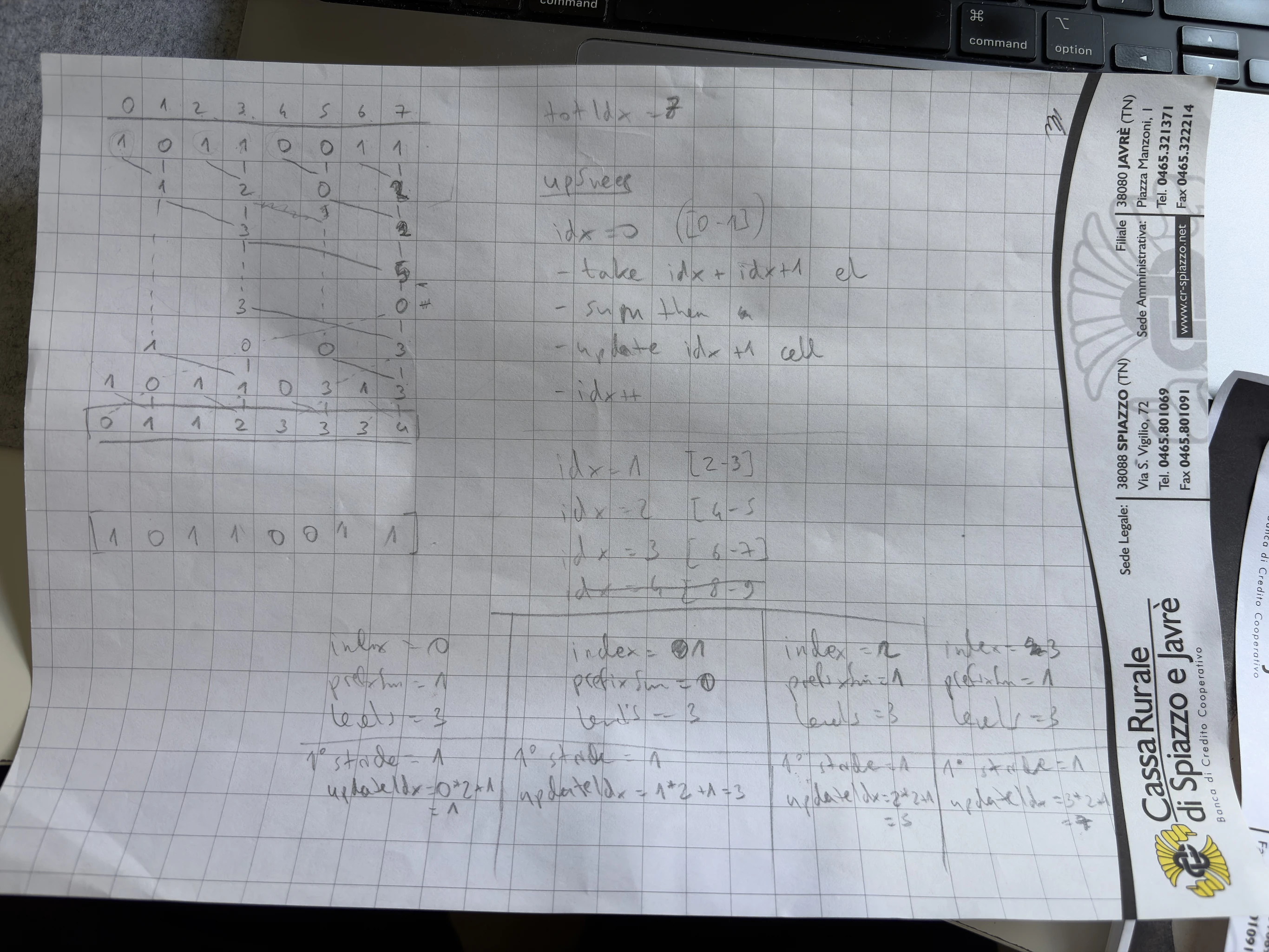
My original Blelloch scan notes, untouched since then :)
Before looking at the algorithm itself, there are three related terms worth separating because I often found them used very close to one another:
- Blelloch scan → calculates the prefix sum in parallel, producing the total number of visible blades at the root along the way
- prefix sum, or scan → gives every visible blade its output position
- stream compaction → writes those blades into their positions, producing a contiguous output
In short:
Blelloch scan → prefix sum → stream compaction → contiguous output
The atomic counter from the previous chapter was already performing stream compaction. It gave every visible blade a unique output position, but they all had to update the same shared counter to get one. The prefix sum is another way to generate those positions in parallel without using that shared counter.
All together now
What helped me make sense of Blelloch scan was relating its shape to the more familiar merge sort algorithm. The two do very different jobs, but they have a similar structure and rhythm.
Both start with pairs, combine them into groups of four, then eight, and continue until everything meets at the end. The difference is that merge sort combines sorted groups, while Blelloch scan combines partial sums.
Same structure, different process.
Just like in merge sort, every group on the same level can be processed independently. That familiar property is crucial here because it allows the GPU to process many groups in parallel before moving to the next level. Once the total reaches the top, Blelloch scan does something merge sort does not: it travels back down through the same structure, distributing the prefixes along the way.
That structure is also what I was trying to capture in my notes above.
It helps to picture Blelloch scan as a tree: the up-sweep is on the left and the down-sweep is on the right. We start at the leaves on the left, move towards the root in the middle, then descend towards the leaves on the right to produce the scan.
That was simpler for me to imagine, but on screen and paper I found it easier to reason about each side as a stacked sequence of levels. That is the framing I will use below.
Here is the complete input and the result we are trying to produce:
blades:      A  B  C  D  E  F  G  H
visibility:  1  0  1  1  0  0  1  1  // 1 = visible, 0 = not visible
scan:        0  1  1  2  3  3  3  4  // result
The scan row is an exclusive prefix sum. Exclusive means that the visibility of the current blade is not included in its
value. Each number answers one question:
How many visible blades came before this blade?
The
scanrow may look sorted, but nothing was compared or reordered. It only increases because the visibility flags are either0or1. The accumulated count can stay the same or go up, but never down.
Producing that result sequentially from left to right would be fairly straightforward. Blelloch scan instead calculates it in parallel through two phases: the up-sweep and the down-sweep.
The up-sweep collects partial sums until they meet at the root (left side of the tree). The down-sweep then distributes those sums back through the same structure until every blade receives its prefix (leaves on the right side of the tree).
Up-sweep
During the up-sweep, neighbouring values are added in pairs. The resulting totals are combined again into fewer, progressively larger groups until everything meets at the root.
blades:      A   B   C   D   E   F   G   H
visibility:  1   0   1   1   0   0   1   1
             └───┤   └───┤   └───┤   └───┤
level 1:         1       2       0       2    // 1 + 0, 1 + 1, 0 + 0, 1 + 1
                 └───────┤       └───────┤
level 2:                 3               2    // 1 + 2, 0 + 2
                         └───────────────┤
root:                                    5    // 3 + 2
At level 1, neighbouring pairs are added together. At level 2, those pair totals are combined into groups of four. The final
addition produces 5, the total number of visible blades.
One level still has to finish before the next one begins, but we no longer need one ordered step for every blade.
The root gives us the total, but it does not yet tell us how many visible blades came before each position. That is what the down-sweep calculates.
Down-sweep
Before the down-sweep begins, the root contains 5, the total number of visible blades. We save it because it will later become
the instance count for the indirect draw. Then we replace the root with 0. This is the identity for addition, but it also has a
useful meaning here: nothing comes before the complete array.
At every stage of the down-sweep, each value is the prefix of the group it represents. It tells us how many visible blades come
before that group begins. The complete array, A..H, begins with 0. When we divide it, A..D still has 0 visible blades before
it, while E..H has 3 because the up-sweep found three visible blades in A..D. This continues until every group contains a
single blade.
From there, every group is divided into a left child and a right child:
- The left child inherits the prefix of its parent.
- The right child receives that prefix and adds to it the up-sweep total of its left sibling.
blades:      A   B   C   D   E   F   G   H
root:                                    0    // 0 before A..H
                         ┌───────────────┤
level 2:                 0               3    // 0 before A..D, 3 before E..H
                 ┌───────┤       ┌───────┤
level 1:         0       1       3       3    // 0 before A..B, 1 before C..D, 3 before E..F, 3 before G..H
             ┌───┤   ┌───┤   ┌───┤   ┌───┤
scan:        0   1   1   2   3   3   3   4    // 0 before A, 1 before B, 1 before C, 2 before D, 3 before E, 3 before F, 3 before G, 4 before H
At level 2, A..D inherits the root prefix of 0. E..H begins after A..D, which the up-sweep found to contain three visible
blades, so it receives 0 + 3.
At level 1, A..B inherits 0, while C..D receives 0 + 1, using the up-sweep total of A..B. On the other side, E..F
inherits 3, while G..H receives 3 + 0 because E..F contains no visible blades.
The same rule applies at every level until we reach the leaves. The values at those leaves form the exclusive prefix sum:
blades:      A  B  C  D  E  F  G  H
visibility:  1  0  1  1  0  0  1  1
scan:        0  1  1  2  3  3  3  4
Before A, there are no visible blades. Before D, there are two. Before H, there are four. The up-sweep collected the partial
sums, while the down-sweep distributed the correct prefix to every position.
Know your place
With the prefix scan done, most of the work is already behind us.
Every visible blade now knows how many visible blades came before it, and along the way we also found the total number of visible blades.
An array index already tells us how many elements come before it. Nothing comes before output[0], one element comes before
output[1], three come before output[3], and so on.
That gives every scan value a convenient second meaning. For a visible blade, it is also the exact position where that blade belongs in the compacted output.
blades:      A  B  C  D  E  F  G  H
visibility:  1  0  1  1  0  0  1  1
scan:        0  1  1  2  3  3  3  4
index:       0  -  1  2  -  -  3  4  // - = does not write because visibility is 0
Some scan values are repeated, true. Both B and C, for example, receive 1. This does not create a collision because B is not
visible and does not write anything. Only C uses that position.
The same happens with E, F and G. They all receive 3, but only G survived the visibility check.
Every visible blade therefore has a unique destination:
A -> output[0]
C -> output[1]
D -> output[2]
G -> output[3]
H -> output[4]
Writing the blades into those positions produces the compacted stream:
output:      A  C  D  G  H  *  *  *
count:       5

* means whatever was there before, it doesn't matter
The total saved before the down-sweep, 5, becomes the instance count in the indirect buffer.
The renderer now has both things it needs: a contiguous list of visible blade indices and the exact number of entries to draw.
Conceptually, this is the same result as the atomic approach from the previous chapter. The difference is how those positions were assigned. The atomic counter handed them out one at a time, while the prefix sum calculated them in parallel beforehand.
Eight values were the friendly version
I used eight values on my piece of paper because it was a small enough number to follow step by step, even manually.
The grass field in Revo has 1,048,576 blades, arranged in a 1024 × 1024 grid. A completely different scale.
Both counts happen to be powers of two (huehue).
The scan itself is not restricted to them, but the clean tree-shaped version we have been following expects every level to split evenly. Luckily, that is easy to fix.
If your visibility list does not contain a power-of-two number of entries, pad its end with zeros until it reaches the next one. If we had five blades, for example, we would add three visibility flags to reach eight:
original visibility:  1  0  1  1  0
padded visibility:    1  0  1  1  0  0  0  0  // three zeros added at the end
Now the tree is full and the scan can continue exactly as before. The padded entries have a visibility of 0, so they add nothing
to the scan and never write into the compacted output.
A small, surgical adjustment :)
Getting the visibility list into shape is the easy part. Handling one million values is a problem of its own, and not a trivial one.
When the GPU runs a compute shader, it does not launch all one million threads as one enormous group. It divides them into smaller
workgroups. In Revo, each workgroup contains 64 threads, with one thread processing one blade.
For 1,048,576 blades, that gives us:
1 compute dispatch
└── 16,384 workgroups
    └── 64 threads each
        = 1,048,576 blades
The 64 is the workgroup size I use here, not a universal WebGPU limit. It is also the Three.js default, which I kept explicitly
in Revo’s config. WebGPU’s default limit for the total number of threads per workgroup is 256, although the selected GPU device
may expose a different limit. The browser validates the shader against that device’s limits.
There is a limit because a workgroup runs as one small, coordinated unit. Its threads need to fit within finite GPU execution
resources and share a limited amount of fast local memory. WebGPU provides 16 KB of this shared workgroup memory by default. A
workgroup containing one million threads could not fit into those resources.
I have not explored this side extensively or benchmarked different workgroup sizes.
A size of 1 would create 1,048,576 tiny workgroups, throwing away most of the benefit of grouping the work. A size of 256 would
reduce that to 4,096 larger groups, but fewer groups do not automatically mean better performance. Larger groups require more GPU
resources at once, while smaller groups introduce more scheduling overhead.
Conveniently, 64 divides the blade count evenly, stays comfortably within WebGPU limits and already performs well for this
workload, so I had no reason to change the default. It remains a configurable constant on purpose so maybe one day I might reopen
this front.
Threads inside one workgroup can also share local memory and wait for one another at a barrier, but separate workgroups cannot. They may run at different times or in a different order, so there is no barrier inside one dispatch that can stop all 16,384 workgroups and make them wait for each other.
That is perfectly fine for my regular grass update because every blade can easily be processed independently.
Blelloch scan is different. Every level depends on the totals produced by the previous one, and those dependencies eventually cross workgroup boundaries.
The complete scan therefore has to be built as a hierarchy of smaller scans:
- Scan each block independently and save its total.
- Scan the smaller list of block totals, repeating if necessary.
- Add the resulting offsets back into each block.
- Scatter the visible blades and write the final draw count.
It is still the same idea, only repeated at different scales. My implementation unfortunately never made it cleanly through those scales, but at least the eight values on my piece of paper did :)
Closing thoughts
Well, that became considerably more than a small trim :)
The previous article ended with me saying I might give real culling another try someday, “if not out of necessity, then perhaps out of sheer curiosity”. Turns out I needed both. Performance gave me the reason to return, while curiosity gave me enough energy to walk into the same problem again knowing I could fail.
I did fail at the prefix-sum version, at least for now. I also stopped dismissing the atomic approach without measuring it, and that was enough to finally ship real GPU culling. Revo is back at 120 FPS in the place that kept dropping to 100, with most of the grass never reaching the vertex stage at all.
A lot of what I know about this corner of graphics came from people writing down what they struggled with. That is also why I still wanted to explain the prefix-sum version properly. If it helps the idea click a little sooner for someone else, it did its job.
I am fully aware of how quickly AI is progressing. It can already help with an incredible number of things and, with the right guidance, it could probably build large parts of something like Revo. I have no interest in pretending otherwise.
Still, I enjoy learning. I want to understand what I am building, not only arrive at the result. Sharing what I learn might help someone wrestling with the same concept, but it also forces me to examine what I think I know and makes that knowledge stick.
AI is a powerful tool. Knowledge is still strength, curiosity is still a superpower, and I have no intention of letting either go hungry.
For now the grass is dense, stable and cheap enough to stop thinking about, which is probably the nicest thing I can say about any system I maintain.
Now I should probably stop staring at it for a little while. I feel a certain urgency to finish watching My Hero Academia in the next couple of months. I think I am somewhere in its second half now and I am loving it :D

Finishing Vinland Saga would be nice too, and I still have some of the Yotei Six to butcher.
Plenty to keep me busy, although the next rabbit hole may already have found me ;)
As with last time, everything described here lives in the Revo codebase. The grass now has a folder of its own, while the schedulers and wind systems should also be easy to find. It is not meant as a reference implementation, but it might be useful to see how the pieces connect in the real project.
Grass folder (may be subject to changes)
Explore more
A few resources that shaped this round of work:
Blelloch Scan - Intro to Parallel Programming - Udacity
Ghost of Tsushima Procedural Grass - GDC Vault
GPU Gems 3, Chapter 39: Parallel Prefix Sum (Scan) with CUDA
WebGPU Specification - W3C
How Do Games Render So Much Grass? - Acerola
Modern Foliage Rendering - Acerola
What I Did To Optimize My Game’s Grass - Acerola
Prefix Sums and Their Applications - Guy E. Blelloch